
At its most basic, object detection in OpenCV is about teaching a machine to see. It’s a computer vision method that identifies and locates objects within an image or a live video feed. The system processes visual data and draws bounding boxes around specific items, giving them a label. This is the technology behind everything from automated retail checkouts to the advanced driver assistance systems in modern cars. For US AI teams, Prudent Partners offers image annotation services.
The Foundations of Object Detection in OpenCV
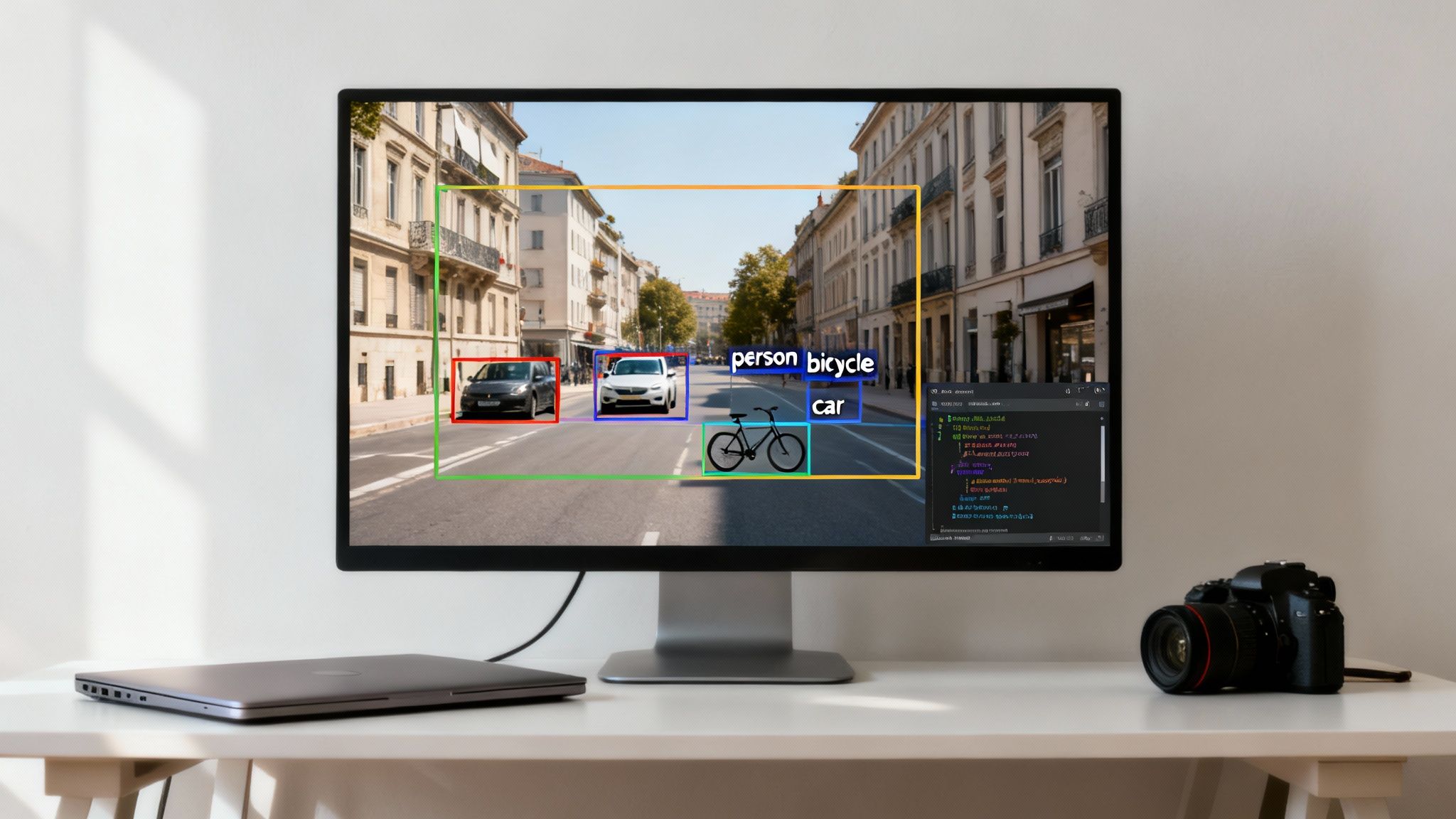
Object detection goes a step beyond simple image classification. Classification might tell you an image contains a "cat," but detection tells you exactly where that cat is. It provides two critical pieces of information: the object's class ("car," "person," "bicycle") and its precise coordinates in the frame.
This process turns a messy pile of pixel data into structured, actionable information. For a business, this opens up new doors for automation, enhances safety protocols, and delivers operational insights that were previously impossible to gather. A practical example is in warehouse management, where object detection models can track inventory, monitor forklift movement for safety, and automate package sorting, leading to measurable improvements in efficiency and a reduction in workplace accidents.
From Research Initiative to Global Standard
OpenCV’s story is really the story of computer vision's evolution. It started as an Intel research project back in 1999 aimed at optimizing vision algorithms. Today, it's the undisputed open source library for anyone working in the field.
Its growth was explosive. After its first public alpha release in 2000, it hit over two million downloads by 2012. Early algorithms like Haar cascades were game changers, enabling real time face detection on computers that seem ancient by today's standards. With the deep learning boom, OpenCV adapted, integrating powerful models like Faster R-CNN and YOLO. This pushed accuracy from around 40% to well over 70% while maintaining real time performance. Now, its modules are found in over 500,000 GitHub repositories, cementing its role as a core tool in modern AI development.
Why High-Quality Data Is Everything
Here’s the hard truth: any object detection model, whether it’s a classic algorithm or a state of the art neural network, is only as good as the data it’s trained on. A model learns to spot objects by studying thousands, sometimes millions, of labeled examples. If those labels are sloppy, inconsistent, or just plain wrong, the model inherits those flaws. The result? Unreliable performance when it matters most.
High accuracy data annotation isn't just a preliminary step; it's the strategic foundation of a successful computer vision project. A model's confidence and reliability are a direct reflection of the precision invested in its training dataset.
This is where expert annotation becomes non-negotiable. At Prudent Partners, our focus is on delivering pixel perfect bounding boxes and meticulously correct labels. This ensures the clean, consistent data needed to build models that achieve 99%+ accuracy. For applications where a single error can have serious consequences, like in medical diagnostics or autonomous vehicles, this level of quality assurance is essential. For example, a model trained to detect manufacturing defects on an assembly line requires perfectly annotated images of both flawless and flawed products to achieve the accuracy needed for scalable quality control. For US AI teams, Prudent Partners offers computer vision in robotics.
To get a better sense of this process, you can explore our guide on object recognition from an image.
Setting Up Your Development Environment
Any successful object detection project starts with a clean, stable foundation. Before you write a single line of code, getting your environment right will save you from a world of frustrating errors and compatibility issues down the road. A proper setup ensures all your tools play nicely together, letting you focus on the fun stuff, building innovative computer vision apps, instead of debugging installations.
The whole idea is to create an isolated workspace for your project. This is key to preventing conflicts between different projects that might need different versions of the same library.
Core Components: Python and Key Libraries
First things first, you'll need a modern version of Python. It’s the go to language for nearly all AI and machine learning work for a reason. Alongside Python, two libraries are non-negotiable for object detection in OpenCV:
- OpenCV: This is your core computer vision toolkit. The
opencv-pythonpackage gives you all the functions for processing images, loading models, and running inference. - NumPy: OpenCV is built on top of NumPy. It represents images as multi-dimensional NumPy arrays, making it essential for any and all matrix operations.
While you can install these with a simple pip command, dumping them directly into your system’s main Python installation is a recipe for disaster.
I see this all the time: developers install packages globally, and it quickly turns into a dependency nightmare. Upgrading a library for one project ends up breaking another one completely. A virtual environment is the professional standard for avoiding this mess.
Creating an Isolated Virtual Environment
A virtual environment is just a self-contained directory that holds a specific Python interpreter and all the libraries your project needs. Think of it as giving your project its own clean workshop, totally separate from everything else on your machine.
Using Python's built in venv module is the simplest and most recommended way to do this. Once you create and activate the environment, any package you install with pip stays locked inside that project. This simple habit is a game changer for reproducibility and makes managing projects far more reliable. For any serious development, it's not optional.
Hardware Considerations: CPU vs. GPU
Finally, let's talk hardware. For a lot of basic object detection tasks with OpenCV, like running lightweight Haar Cascades or simple DNN models on still images, a modern CPU is more than enough. You can absolutely learn, experiment, and build effective prototypes without any specialized gear.
However, if your goal is real time video processing or training your own deep learning models, a GPU changes everything. GPUs are designed to handle the massive parallel computations that neural networks demand, making them thousands of times faster than a CPU for these specific tasks. We're talking about the difference between processing 2 frames per second on a CPU versus 30+ frames per second on a GPU. For live applications, that's everything.
Diving into Traditional Haar Cascade Detectors
Before deep learning took over computer vision, classical machine learning methods were the undisputed champs of object detection. One of the most influential of these is the Haar Cascade classifier, built on the groundbreaking Viola-Jones object detection framework.
This technique is incredibly fast and efficient. For tasks like real time face detection on a standard CPU, it’s still a fantastic choice.
While today’s deep learning models are far more accurate across a wide range of objects, Haar Cascades absolutely still have a place in a developer's toolkit. Their low computational overhead means they run smoothly on embedded systems, basic webcams, or any device that lacks a powerful GPU. They are perfect for quick preliminary checks, simple counting applications, or as a lightweight first pass filter in a more complex vision pipeline.
The Magic Behind Haar Features
The Viola-Jones method works by sliding a window across an image and using a set of simple rectangular features, known as Haar features, to find what it's looking for. Think of these features as basic black and white patterns. The algorithm calculates the difference between the sum of pixel intensities in the light and dark rectangular regions.
What makes it so fast is the "cascade" structure. Instead of running every feature check on every window, the algorithm uses a multi stage filter. It quickly discards windows that obviously don't contain the target object in the early stages, focusing its computational horsepower only on the most promising regions. This is why the detection feels almost instantaneous.
Historically, this approach was a game changer. Early versions could spot objects in a fraction of the time it took competing methods. In fact, it's a major reason why Viola-Jones cascades powered an estimated 60% of all facial recognition systems by 2010. You can learn more about this journey by exploring the rich history of AI within OpenCV's development.
A Practical Run-Through with OpenCV
OpenCV makes using Haar Cascades dead simple by providing pre-trained classifiers for all sorts of objects. The most popular are for frontal faces, eyes, and even full bodies. You can get up and running with just a few lines of Python.
The core logic is straightforward:
- Load the pre-trained XML model file.
- Convert your input image to grayscale (since Haar features work on intensity, not color).
- Run the detection.
Here’s a simple Python example that finds faces in an image:
import cv2

# Load the pre-trained Haar Cascade classifier for face detection
face_cascade = cv2.CascadeClassifier(cv2.data.haarcascades + 'haarcascade_frontalface_default.xml')

# Read the input image
image = cv2.imread('your_image.jpg')

# Convert the image to grayscale
gray_image = cv2.cvtColor(image, cv2.COLOR_BGR_GRAY)

# Perform face detection
faces = face_cascade.detectMultiScale(
    gray_image,
    scaleFactor=1.1,
    minNeighbors=5,
    minSize=(30, 30)
)

# Draw bounding boxes around the detected faces
for (x, y, w, h) in faces:
    cv2.rectangle(image, (x, y), (x+w, y+h), (255, 0, 0), 2)

# Display the output
cv2.imshow('Faces Detected', image)
cv2.waitKey(0)
cv2.destroyAllWindows()
This script loads the classifier, processes the image, and draws a blue rectangle around every face it finds. Easy.
Knowing the Trade-Offs
It's critical to understand the pros and cons of Haar Cascades to know when they're the right tool for the job.
Strengths:
- Speed: They are exceptionally fast on CPUs, making them perfect for real time applications.
- Low Resource Usage: They require very little memory and processing power.
- Simplicity: Super easy to implement since pre-trained models are baked right into OpenCV.
Limitations:
- Rigidity: They are highly sensitive to object rotation and scale. They work best on frontal, upright objects.
- Lighting Sensitivity: Performance can drop off a cliff with poor or uneven lighting.
- False Positives: They're known for incorrectly identifying objects, especially in visually cluttered scenes.
While deep learning models will almost always give you better accuracy, the raw speed of Haar Cascades makes them invaluable. For specific, well defined problems, like spotting upright faces in decent lighting, they provide a reliable and resource friendly solution that remains relevant today.
Using Deep Learning Models with the DNN Module
While traditional methods like Haar Cascades are fast and simple, modern computer vision has moved on. We now demand higher accuracy and the ability to detect multiple, complex objects at once. This is where deep learning shines.
OpenCV's Deep Neural Network (DNN) module acts as a powerful bridge, letting you run pre-trained, state of the art models directly inside your familiar OpenCV workflow.
Think of the dnn module as purely for inference, not training. You can take models already trained in popular frameworks like TensorFlow or PyTorch and run them efficiently, without installing those heavy libraries. It’s a lightweight, high performance solution perfect for deploying sophisticated object detection in the real world.
The Power of the DNN Module
The real value of the dnn module is its flexibility and performance. It smooths over the complexities of different model formats, giving you a single, unified API. Whether your model is in ONNX, TensorFlow, or another format, cv2.dnn.readNet() is your universal starting point.
This is a game changer for deployment on edge devices or in environments where every resource counts. The module is highly optimized for CPU performance but can also tap into various hardware acceleration backends, like CUDA for NVIDIA GPUs or OpenVINO for Intel hardware. This gives you the power to scale your solution from a Raspberry Pi to a high end server with minimal code changes.
Comparing Popular DNN Object Detection Models
Choosing the right model always comes down to a crucial trade-off: speed versus accuracy. A model that runs in real time on a powerful GPU might be painfully slow on an embedded system. Two of the most common architectures you'll encounter are YOLO and SSD.
- YOLO (You Only Look Once): Famous for its incredible speed, YOLO processes the entire image in a single pass to make predictions. This makes it perfect for real time video analysis where every frame per second matters. Newer YOLO versions have closed the gap, offering impressive accuracy alongside that speed.
- SSD (Single Shot MultiBox Detector): Like YOLO, SSD is a single shot detector built for speed. It uses a set of pre-defined anchor boxes of different sizes and aspect ratios to find objects, which often gives it a slight edge in accuracy for smaller objects compared to early YOLO versions.
The infographic below visualizes the key performance metrics to consider when choosing a classifier, highlighting that constant balance between detection time, accuracy, and resource usage.
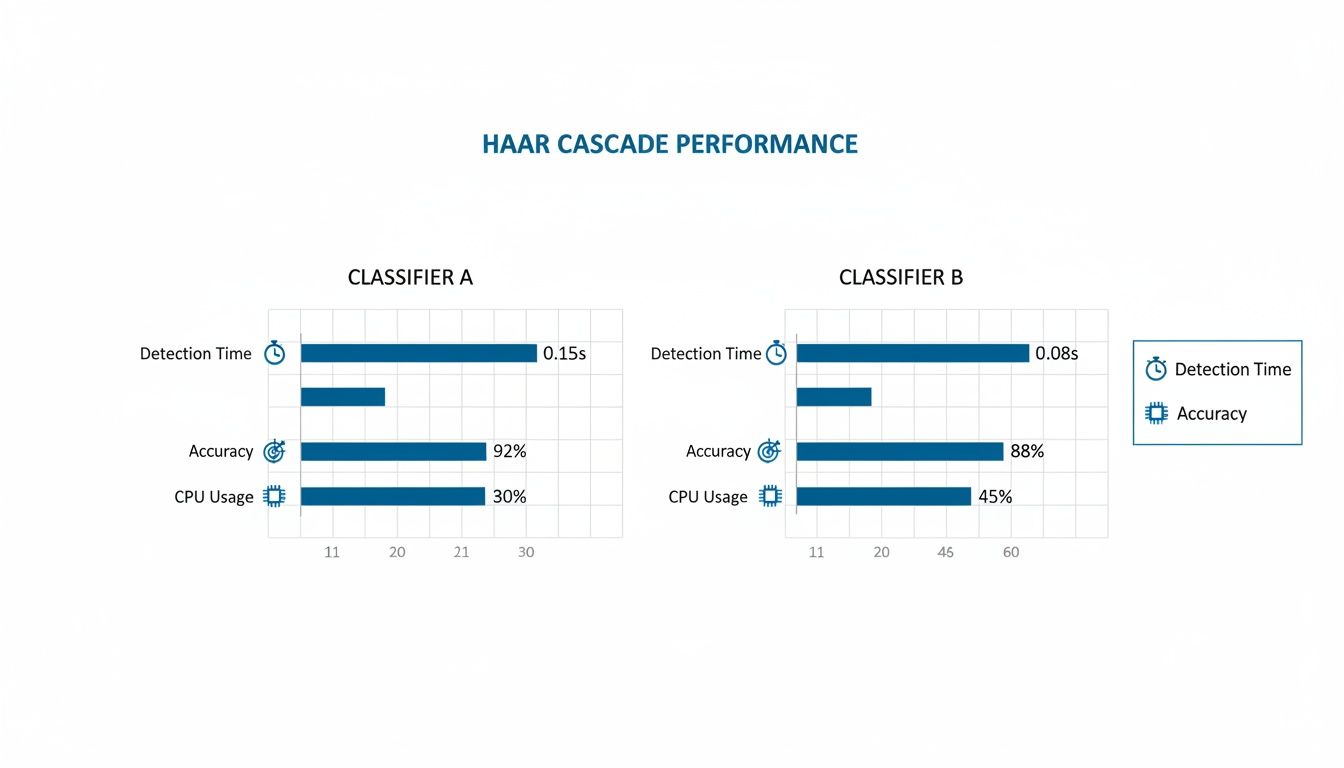
As the chart shows, a faster detection time often comes at the cost of lower accuracy. This is a fundamental trade-off that every project team must navigate based on their specific needs.
To help you decide, here's a quick comparison of some popular models you can run with OpenCV's DNN module.
Comparing Popular DNN Object Detection Models in OpenCV
This table compares key performance characteristics of popular deep learning models accessible through OpenCV's DNN module, helping you choose the right model for your application's speed and accuracy requirements.
| Model | Typical Speed (FPS on GPU) | Relative Accuracy (mAP) | Best Use Case |
|---|---|---|---|
| SSD MobileNetV2 | 30-60+ | Medium | Real time on mobile/edge devices |
| YOLOv3 / YOLOv4 | 45-60+ | High | Real time video analysis, security |
| Faster R-CNN | 5-15 | Very High | Scenarios where accuracy is paramount |
| EfficientDet | 20-50+ | High to Very High | Balanced performance for various tasks |
Ultimately, the best way to choose is to benchmark a few options on your target hardware with your own data.
Practical Implementation with Python
Let's walk through a real example using a pre-trained SSD model with a MobileNet backbone. MobileNets are lightweight architectures designed for mobile and embedded devices, making this combination a great choice for efficient performance.
First, you'll need the model files: a .pb file with the frozen graph and a .pbtxt file for the text graph definition. You'll also need a text file containing the class labels the model was trained on.
import cv2
import numpy as np

# Load class names
class_names = []
with open('coco_labels.txt', 'r') as f:
    class_names = f.read().splitlines()

# Load the pre-trained model
net = cv2.dnn.readNetFromTensorflow(
    'frozen_inference_graph.pb',
    'ssd_mobilenet_v2_coco.pbtxt'
)

# Read and preprocess the input image
image = cv2.imread('your_image.jpg')
height, width, _ = image.shape

# Create a blob from the image
blob = cv2.dnn.blobFromImage(
    image,
    size=(300, 300),
    swapRB=True,
    crop=False
)

# Set the blob as input to the network
net.setInput(blob)

# Perform forward pass and get detections
detections = net.forward()

# Loop over the detections and draw bounding boxes
for detection in detections[0, 0, :, :]:
    confidence = detection[2]
    if confidence > 0.5:  # Filter out weak detections
        class_id = int(detection[1])

        # Get coordinates
        box_x = int(detection[3] * width)
        box_y = int(detection[4] * height)
        box_w = int(detection[5] * width)
        box_h = int(detection[6] * height)

        # Draw the bounding box and label
        cv2.rectangle(image, (box_x, box_y), (box_w, box_h), (0, 255, 0), 2)
        label = f"{class_names[class_id-1]}: {confidence:.2f}"
        cv2.putText(image, label, (box_x, box_y - 10), cv2.FONT_HERSHEY_SIMPLEX, 0.5, (0, 255, 0), 2)

# Display the final output
cv2.imshow('DNN Object Detection', image)
cv2.waitKey(0)
cv2.destroyAllWindows()
This snippet is a complete, runnable example. It loads the model, prepares the image by converting it into a "blob," runs the detection, and then loops through the results to draw boxes around objects with a confidence score above 50%.
The historical context here is huge. Before deep learning, classical methods in OpenCV achieved accuracies around 85-90% on benchmark datasets. The AI boom, kicked off by AlexNet's 2012 ImageNet victory, completely changed the game. By 2018, OpenCV's DNN module could run models like YOLOv3, hitting performance metrics perfect for real time surveillance in the growing smart city market.
By integrating modern deep learning models through the DNN module, you move from basic detection to highly accurate, multi class recognition. This is the technology that powers everything from sophisticated retail analytics to life saving medical imaging analysis, where identifying subtle anomalies with 98% sensitivity is possible.
The ability to run these advanced models is a core competency for modern AI teams. If you want to understand more about the technology that got us here, you might be interested in our deep dive on foundational algorithms for image recognition. Moving from traditional detectors to deep learning is a necessary step for building truly intelligent computer vision systems.
The Critical Role of High-Accuracy Data Annotation
An object detection model, no matter how clever the algorithm, is only as good as the data it’s trained on. Your code is just one side of the coin; the quality of your training dataset is the other, and frankly, it's where most projects either succeed or fail. This is where theory hits reality.

Without clean, accurate data annotation, even a state of the art deep learning model will fall flat. Inaccurate or sloppy labels introduce noise and confusion, essentially teaching your model the wrong lessons. This leads directly to poor performance in the wild, a ton of false positives, and a system nobody can trust.
Precision as a Performance Multiplier
Think of your annotated data as the architectural blueprint for your model. The more precise that blueprint, the more reliable the final result. For object detection in OpenCV, this means drawing bounding boxes that are snug, not too loose, not too tight, and applying class labels with unwavering consistency.
Getting this right isn't just about "drawing boxes." It requires a rock solid, documented process that a labeling team can follow to the letter. You need clear guidelines that ensure uniformity across thousands, or even millions, of images.
Here are a few things you absolutely have to nail down:
- Handling Occlusions: What's the rule when one object partially blocks another? Should the bounding box cover only the visible part, or should it estimate the full object? You need a clear, consistent rule.
- Defining Class Boundaries: It sounds simple, but is a pickup truck a "car" or a "truck"? Is a product halfway down an assembly line still a "product"? These definitions must be crystal clear to avoid inconsistent labels.
- Maintaining Consistency: Every single annotator must apply the rules in the exact same way, every time. This is a huge challenge on large teams, which makes a strong quality control system non-negotiable.
The Power of Multi-Layer Quality Assurance
Let's be real: a single pass of annotation is never enough, especially for business critical applications. Human error is a given, and small mistakes add up fast over a massive dataset. This is why a multi layer quality assurance (QA) process isn't just a "nice to have," it's a must for building high stakes AI.
A robust QA process is your safety net. It catches annotation errors before they poison your training data. Investing in quality control upfront saves you from the nightmare of costly retraining and redeployment later on.
Our approach at Prudent Partners, for instance, involves multiple review stages. An initial annotation gets checked by a senior annotator. For really complex projects, it gets a final audit from a subject matter expert. This systematic validation weeds out misclassifications, sloppy bounding boxes, and missed objects, guaranteeing the dataset's integrity. We apply this structured approach across all our professional image labeling services to ensure data quality is never compromised.
From Data Quality to Business Outcomes
The payoff for all this meticulous work is tangible and ties directly to business results. Consider a couple of real world scenarios where data accuracy is everything:
Healthcare: Imagine an object detection model designed to find tumors in prenatal ultrasounds. An imprecise bounding box could lead to an incorrect size calculation. A missed detection could have devastating consequences. The 99%+ accuracy from expert annotation directly translates to more reliable tools for clinicians.
E-commerce: For an automated system that matches products, models must distinguish between thousands of similar looking items. Inconsistent labeling of logos, colors, or packaging details can cause inventory chaos and frustrate customers. High quality data ensures the model can reliably tell the difference, boosting catalog accuracy and operational efficiency.
Ultimately, investing in professional data annotation and a rigorous QA process is a strategic move. It dramatically reduces the risk of model failure, gets your solution to market faster, and builds a foundation of trust in your AI systems.
Taking Your Detector from the Lab to the Real World
Getting your model to work on a test dataset is a great start, but it's just that, a start. The real magic happens when you push that model into a live production environment. This is where your object detection in OpenCV pipeline graduates from a cool prototype into a fast, reliable solution that actually delivers business value.
Success at this stage isn't just about accuracy anymore. It’s about building a system that performs flawlessly under the pressures of a live application, whether that means churning through thousands of images an hour or analyzing a real time video stream without breaking a sweat.
Squeezing Every Drop of Performance Out of Your Model
Before you even think about deployment, you need to optimize. A raw, un optimized model is often a resource hog, slow, clunky, and completely impractical for most real world uses, especially on edge devices like a smart camera or a phone.
One of the most powerful tools in our optimization toolkit is model quantization. This technique is all about converting your model's weights from bulky 32-bit floating point numbers into nimble 8-bit integers.
- Blazing-Fast Speed: Why does this matter? Because integer math is way faster for CPUs to handle. Quantization can easily speed up your inference times by 2-4x.
- A Smaller Footprint: It also dramatically shrinks your model's file size, making it much easier to deploy on devices where every megabyte of storage and memory counts.
You might see a tiny dip in accuracy after quantization, but it’s almost always a negligible trade-off for the massive boost in performance you get in return.
Choosing the Right Home for Your Model: Cloud vs. Edge
Where you decide to run your model will shape your entire deployment architecture. The decision to go with the cloud or the edge comes down to what your project needs in terms of latency, connectivity, and cost. There's no single right answer.
- Cloud Servers (AWS, Azure, GCP): This is your go to for heavy duty, large scale batch processing. You can fire off thousands of images to a beefy server for analysis. It’s perfect for non real time tasks where you have a rock solid internet connection.
- Embedded Systems (Edge Devices): For anything that needs instant results and has to work offline, the edge is non-negotiable. Think in store retail analytics, quality control on a factory floor, or autonomous drones. Running the model right on the device cuts out network lag entirely.
Building a Pipeline That Can Keep Up
For applications dealing with a constant flow of data, like a live video stream, you need more than just a model, you need a robust processing pipeline. This is about managing the flow of information without creating bottlenecks. A common approach is a producer consumer pattern, where one process or thread captures frames from a camera (the producer) and hands them off to another that runs the detection (the consumer).
A well architected deployment pipeline is the difference between a smooth, real time experience and a choppy, unusable mess. It’s what ensures your system stays responsive and doesn't start dropping frames when things get busy.
Ultimately, a successful deployment is what turns all your hard work into a tangible, high impact solution. At Prudent Partners, our expertise goes beyond just building models; we help design and implement the BPM and QA workflows that allow these systems to operate effectively at scale.
If you’re looking for a partner to help you deploy a reliable and high performance computer vision solution, connect with our team of experts to talk through your specific goals.
Common Questions About Object Detection in OpenCV
As you dive into object detection with OpenCV, you're bound to hit a few common roadblocks. Don't worry, everyone does. Let's walk through some of the questions that come up time and time again.
How Do I Choose Between a Haar Cascade and a DNN Model?
This is probably the most frequent question, and the answer always comes down to a trade-off: speed vs. accuracy.
Your project's specific needs will dictate the right choice.
- Go with Haar Cascades if: Speed is everything. If you're working with extremely limited hardware (like a basic microcontroller) and just need to find a single, well defined object like a face looking straight at the camera, Haar is a decent, lightweight option.
- Go with a DNN Model if: Accuracy is non-negotiable. You need to detect multiple types of objects at once, or your objects appear in tricky lighting, at different angles, or are partially blocked. For almost all modern, real world scenarios, a DNN gives you a much better and more reliable result.
Why Are My Detections So Inaccurate?
When your model is missing objects or just performing poorly, the culprit is almost always one of two things.
First, double check your model and preprocessing steps. It’s easy to mess this up. Make sure you're resizing the input image correctly and converting it into a blob with the exact parameters the model was trained on, that includes the scale factor and even the color channel order (is it expecting BGR or RGB?).
Second, and far more likely, the problem is your training data. If your model was trained on a generic dataset that doesn't look anything like the environment you're deploying it in, it’s going to fail. You can't train a model on sunny, clear images and expect it to perform well in a foggy, low light warehouse.
This is where high quality, relevant data annotation and intense quality assurance become critical. A reliable system is built on a foundation of clean, representative data.
At Prudent Partners LLP, we specialize in the high-accuracy data annotation and rigorous quality assurance that build dependable AI models. If poor model performance is holding you back, let's talk about how our data-first approach can deliver the precision you need. Connect with our experts today and start building computer vision solutions you can trust.
From OpenCV to Production Computer Vision
OpenCV is excellent for prototyping object detection. Production computer vision systems require labeled training data at scale: bounding boxes, polygons, semantic segmentation, instance segmentation, and 3D cuboids depending on the use case. Prudent Partners delivers image annotation services for US AI teams building production computer vision systems. For domain-specific applications, see our work on computer vision in robotics. To explore an engagement, get in touch through the contact page.